In I reviewed several basic applications for generating fair-value estimates for the Treasury yield, which can be used as a proxy for projecting return. Let’s expand this effort by forecasting performance for the US equity market over a 10-year window. The goal is developing a baseline outlook for a 60/40 US stock/bond portfolio over a 10-year horizon.
In recent updates I outlined three methodologies for modeling fair-value estimates of the 10-year rate and using the average of the three as a forecast. That’s effectively a 10-year return estimate because buying and holding a 10-year Note will more or less generate a total return that’s close to the current yield at the time of purchase.
In fact, no modeling for the 10-year Note is needed to approximate the ex ante 10-year return: current yield will suffice and is almost certainly a better forecast. Nonetheless, the modeling effort offers a reality check of sorts, along with some theoretical perspective. Ideally, fair value matches current yield exactly. In practice, that’s rarely the case and so the divergences offer context for deciding where the 10-year rate may be headed and whether the current yield appears to offer reasonable compensation, given the current macro and markets environment.
As for stocks, projecting return is more challenging and therefore more reliant on modeling efforts. There are many ways to proceed. Let’s start by using the Professor Robert Shiller’s Cyclically Adjusted Price Earnings Ratio (CAPE), a widely monitored valuation measure of the US equity market.
To make this analysis somewhat comparable to the 10-year yield modeling outline previously, we’ll use CAPE data starting in 1971. Note that modeling results will vary depending on the start date, which for CAPE goes back to 1871. Using a much longer time window has merit, but the counterpoint is that a more realistic modeling project will focus on recent decades to reflect how markets are behaving in the modern era. To be fair, a professional consulting project would consider a range of time windows, but in the interest of brevity here we’ll focus on the 1971-plus period.
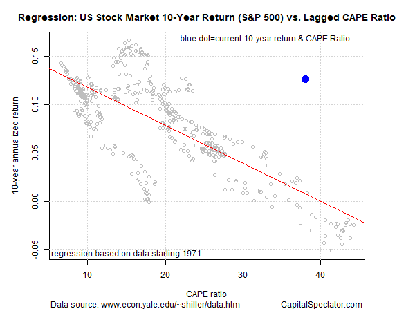
The main result is shown in the graph below, which regresses the 10-year annualized return of the Index against a 10-year lag of the CAPE ratio. In other words, the CAPE ratio of a 10 years earlier is used to estimate the subsequent 10-year change in the US stock market.

US Stock Market 10-Yr Return Vs Lagged CAPE Ratio
As the chart suggests, there’s a relationship between the data. It’s hardly perfect, but there’s a clear implication that higher CAPE ratios align with lower subsequent market returns, and vice versa.
The blue dot shows the current 10-year return and CAPE ratio: 12.6% and 38.0, respectively. Ouch! The blue dot is far above the red regression line. That’s a strong clue for managing expectations down for the S&P’s 10-year return outlook relative to the past 10-year performance. Indeed, the regression modeling estimates that the 10-year market performance will be roughly 1% to 2%.
The caveat, of course, is that the modeling reflects a fair amount of noise and so actual results can and probably will vary relative to the model. The R-squared for the fit in the regression above is roughly 0.58. If the modeling was perfect, the R-squared reading would be 1.0 – i.e., the model explained 100% of the variation in the 10-year returns. At 0.58, by contrast, just shy of 60% of the variation is captured by the model.
That’s still a reasonably strong fit, but it leaves plenty of room for variation, as shown in the chart above via the wide range of fluctuation in the gray circles around the red regression line.
Let’s take a relatively optimistic view of the modeling and assume that the S&P will generate a 2.5% annualized return over the next 10 years. Pairing that with the current 1.37% yield for 10-year Treasury Note suggests that a 60/40 portfolio will earn roughly 2% in the decade ahead – well below the trailing performance for this benchmark portfolio.
In Part II, we’ll model the S&P’s return outlook with a variation of the CAPE ratio that adjusts for the real (inflation-adjusted) Treasury rate.
The goal here is to build three equity-return forecasting models and use the average of the trio to boost the reliability of the projection. Combining forecasts tends to deliver superior results vs. any one forecast. Accordingly, our first attempt to project the S&P’s performance should be viewed with a high degree of caution since it reflects a single modeling effort.

